- Tags:: 📚Books , 🗣️ A chart from the 40s is all you need
- Author:: Donald J. Wheeler
- Liked:: 8
- Link:: https://www.amazon.com/Making-Sense-Data-Donald-Wheeler/dp/0945320728
- Source date:: 2012-05-02
- Finished date:: 2024-03-24
- Cover::
Why did I want to read it?
To prepare 🗣️ A chart from the 40s is all you need.
What did I get out of it?
1. Introduction
The control chart, or Shewhart chart or process behavior chart was invented in the 30s:
The foundation for the techniques of Continual Improvement was laid by Dr. Walter Shewhart, a physicist who worked with Western Electric and Bell Laboratories. His pioneering work in the 1920s was focused on quality in manufacturing. However, his approach is universally applicable, valid with all kinds of data, and useful in all types of organizations. Dr. W. Edwards Deming extended Shewhart’s work by developing and explaining its applications, first in the U.S., then in Japan after World War II, and finally throughout the world in the 80s and 90s (View Highlight)
In his book, Economic Control of Quality of Manufactured Product [1931], Shewhart came up with a way of computing limits to separate routine variation from exceptional variation (View Highlight)
6. Some arithmetic
He says that root mean square deviation and standard deviation could be confusing (different denominator since we divide by n-1 in standard deviation). I don’t think this is true today:
because the range is so simple, it is best to start out with these two measures (View Highlight)
7. Visualize your process behavior
Bar charts and running records provide pictures of your data. In each case you obtain a picture that displays relationships or data in their context. In many cases these contextual displays will be sufficient. (p. 95)
The trick is to strike a balance between the consequences of these two mistakes, and this is exactly what Walter Shewhart did when he created the control chart (…) so that you will have very few false alarms. Shewhart’s choice of limits will bracket approximately 99% to 100% of the routine variation. As a result, whenever you have a value outside the limits you can be reasonably sure that the value is the result of exceptional variation
7.1 Two types of variation
How can you interpret the current value when the previous values are so variable? The key to understanding any time series is to make a distinction between two types of variation. The first type of variation is routine variation. It is always present. It is unavoidable. It is inherent in the process. Because this type of variation is routine, it is also predictable. The second type of variation is exceptional variation. It is not always present. It is not routine. It comes and it goes. Because this type of variation is exceptional, it will be unpredictable.

A process that displays unpredictable variation is changing over time. Because of these changes we cannot depend upon the past to be a reliable guide to the future (View Highlight)
An unpredictable process will possess both routine variation and exceptional variation. (View Highlight)
On the other hand, looking for common causes of routine variation will be a low payback strategy because no single common cause is dominant. (View Highlight)
If we use it for KPIs, we won’t want to remove those causes
Whenever points fall outside the limits, go look for the assignable causes. As you find the assignable causes, and as you take appropriate actions to remove the effects of these assignable causes from your process, you will be improving your process (View Highlight)
The following detection rules, known as run tests, look for weaker signals by using sequences of points. (View Highlight)
Why being so mysterious
for reasons that are beyond the scope of this book, run tests should not be applied to the chart for moving ranges. (View Highlight)
a sequence of eight, nine, or ten successive values that are al on the same side of the central line is generally taken to be evidence of a shift in location (View Highlight)
Another way that a weak but sustained assignable cause can make its presence known on an X Chart is a “run near the limits:” a sequence of three out of four successive values, in the upper (or lower) 25% of the region between the limits (View Highlight)
How can something this simple have an impact upon the whole organization? (View Highlight)
How much do you have? In the preceding example limits were computed at the end of Year Two using only five values and four moving ranges, because that was all the data that was available that was reasonable to use. In practice it is nice if you can use a dozen or even two dozen values to compute your limits (View Highlight)
When values that are known to have come from different cause systems are mixed together on a single running record it is inappropriate to compute limits for that plot (View Highlight)
Virtually every statistical technique for making comparisons between groups, items, or categories is built on the assumption that the data within each category are homogeneous. When this is demonstrably and globally not true, all comparison techniques become arbitrary and capricious. And when your comparison technique is arbitrary and capricious, your results will be no better. (View Highlight)
“These limits are far too wide to be useful.” Are they? It is not the limits that are at fault but rather the noise in the data. The limits in Figure 10.7 are based upon the data given. These limits are wide simply because these data are full of noise. The process behavior chart limits are the Voice of the Process. Whether or not you like the Voice of the Process does not matter to the process (View Highlight)
Shewhart chose to draw the line between routine variation and exceptional variation according to the formula: Average ± 3 Sigma which is why the Natural Process Limits for the individual values, the Upper Range Limit, and those limits which we will encounter later may all be referred to as three-sigma limits (View Highlight)
We do not want to detect each and every little change in the process. It is just those assignable causes whose impact is great enough to justify the time and expense of investigation that we are interested in detecting and removing. We want to detect the strong signals (View Highlight)
A symmetric interval is generic and safely conservative. The term sigma denotes a standard unit of dispersion. “Experience indicates that t = 3 seems to be an acceptable economic value.” Theory suggests that three-sigma limits should filter out virtually all of �he probab �e noise, and experience indicates that three-sigma limits are sufficiently conservative for use m practice. (View Highlight)
Three-sigma limits are not used because they correspond to some theoretical probability. They are used because while they are consistent with theory, they have also been thoroughly proven in practice to be sufficiently conservative. (View Highlight)
The first remarkable thing we can learn from Figure 11 .2 is that in each case the three-sigma limits cover virtually all of the routine variation. This means that we do not have to have a “normally distributed” process in order for the limits to work. Three-sigma limits are completely general, and work with all types of process behaviors (View Highlight)
In practice, skewed distributions occur when the data pile up against a boundary or barrier. This barrier would be on the left in Figure 11.2. Such a barrier precludes any substantial shift toward the lower limit, and effectively makes the lower limit irrelevant (View Highlight)
The objective is not to compute the limits with high precision, but rather to use the limits to characterize the process as being either predictable or unpredictable. (View Highlight)
Three-sigma limits are not used because they correspond to some theoretical probability. They are used because they are consistent with theory and have been thoroughly proven in practice to be sufficiently conservative (View Highlight)
why did we not make use of this common measure of dispersion when we computed limits for the XmR Chart? (View Highlight)
while the XmR Chart examines the data for evidence of nonhomogeneity, the global standard deviation statistic, s, assumes the data to be completely homogeneous. (View Highlight)
Do the exercise
Correctly computed limits will allow you to detect the nonhomogeneous behavior of the data in Table 11.2. You will get the chance to see this for yourself in Exercises 11.1 and 11.2. (View Highlight)
I’m not sure I understand this part: one thing is computing a global summary statistic, and the other is which statistic. Why can’t we use the standard deviation in a small number of points?
In order for the process behavior chart approach to work it has to be able to detect the presence of assignable causes even though the limits may be computed from data which are affected by the assignable causes. In other words, we have to be able to get good limits from bad data. This requirement places some constraints on how we perform our computations. In order to get good limits from bad data with an XmR Chart you will have to use the moving ranges to characterize the short-term, point-to-point variation. The formulas then use this short-term variation to place limits on the long-term variability. This is why limits for an XmR Chart must be computed using either the average moving range or the median moving range. You cannot use any other measure of dispersion to compute limits for an X Chart. Specifically, you cannot use global measures of dispersion to compute limits. This precludes the use of the standard deviation statistic computed on a single pass through all of the data. Whenever the data are affected by assignable causes a global measure of dispersion will always be severely inflated, resulting in limits that will be too wide and a process behavior chart that will be misleading. (View Highlight)
Sonic says: “say no to drugs”
if a stranger, or even a friend, offers you another way of computing limits, just say no! (View Highlight)
 (
(11.4 But How Can We Get Good Limits From Bad Data? (View Highlight)
11.5 So Which Way Should You Compute Limits? (View Highlight)
The average moving range is more efficient in its use of the data than is the median moving range. However, in the presence of one or more very large ranges the average moving range is subject to being more severely inflated than the median moving range. When this happens the median moving range will frequently yield the more appropriate limits. (View Highlight)
11.6 Where Do the Scaling Factors Come From? (View Highlight)
THE ORIGIN OF THE 2.660 SCALING FACTOR (View Highlight)
With an effective subgroup size of two, the value for d2 is 1.128 (see Table 1 in the Appendix). (View Highlight)
3 Sigma(X) = mR 3 d2 = 3 mR lalZB = 2.660 mR (View Highlight)
the charts will err in the direction of hiding a signal rather than causing a false alarm. Because of this feature, when you get a signal, you can trust the chart to be guiding you in the right direction. (View Highlight)
Descriptive summaries may be interesting, but they should never be mistaken for analysis. Analysis focuses on the question of why there are differences. (View Highlight)
In this language, the problem with the typical “analysis” shown in Tables 12.1 to 12.5 is a failure to make any allowance for noise. All differences are interpreted as signals, with the consequence that reprimands and commendations are handed out at random each quarter. (View Highlight)
I would say it is better to detrend first.
Since the limits in Figure 12.2 are 93.5 units on either side of the central line, we place trended limits 93.5 units on either side of the half-average points to get the chart shown in Figure 12.4 (View Highlight)
This can be used in Weekly Business Reports
So what insight is gained by comparing this quarter’s sales with the sales in previous quarters? What do such descriptive percentages accomplish? They only serve to confuse the numerically illiterate (View Highlight)
we have not made any adjustment in the width of the limits when we placed them around a trend line. Shouldn’t we make some adjustment for the trend? In most cases there will not be enough of a change to warrant the effort (View Highlight)
While slightly narrower limits might increase the sensitivity of the chart in Figure 12.6, they will not remedy the situation, and if the trend is not changed, the width of the limits will be a moot point. The objective is insight, with an eye toward improvement, rather than calculating the “right” numbers (View Highlight)
“Wouldn’t a regression line work better? (View Highlight)
Complexity is not a problem to this nowadays.
But here there is no sense in which these trends in sales “depend” upon the time period. The relationships here are not cause-and-effect, but rather coincidental. When this is the case we can use the simple method of half-averages with confidence that we will obtain reasonable trend lines without undue complexity (View Highlight)
Once more the local, limited comparisons mislead rather than inform. (View Highlight)
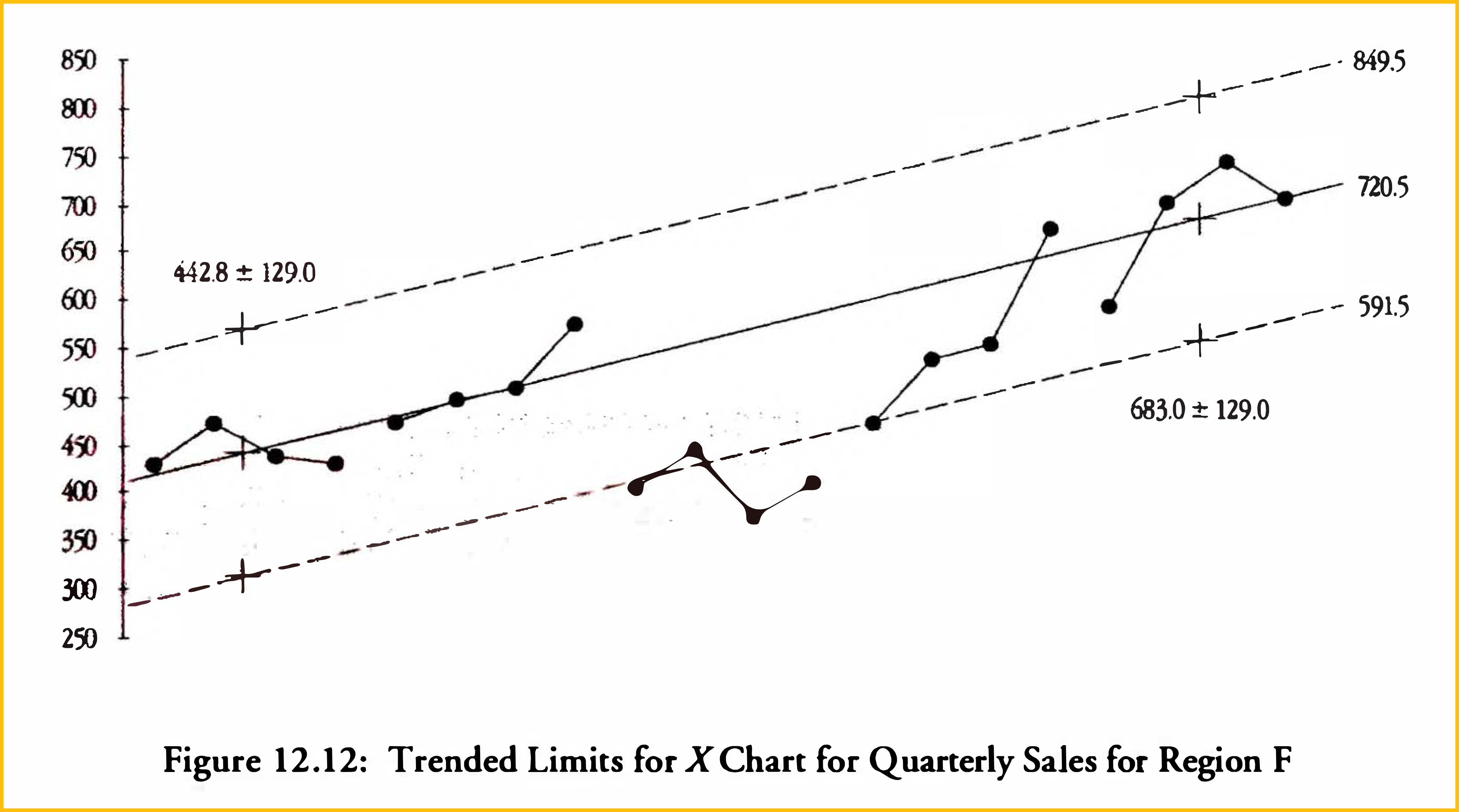
This third estimate of a trend line avoids the depressing effect of the drop from Year Two to Year Three. At the same time it avoids the excessive optimism of using only the last three years. Which is why it is used in Figure 12. 12. If the sales in Region F do better than this, the chart will tell us and we can then revise our trend line. There is always an element of judgment required to use process behavior charts. (View Highlight)
 (
(Time series which consist of the sum of many different components will tend to be more predictable than their components-the whole is more predictable than the parts. As the individual components of a time series are accumulated the noise also accumulates. With each additional component there is more room for the values to average out, leaving a time series that is globally predictable even though the individual components are unpredictable. (View Highlight)
the wide limits do indicate the amount of noise contained in these values. So if you encounter wide limits do not be dismayed. They simply mean that your data contain a lot of noise, which is to be expected with highly aggregated time series (View Highlight)
If you cannot express in words what a computed value represents, then you have left the real � of common sense. (View Highlight)
For example, consider comparing the number of transactions on successive days of the week. The number of transactions per day might vary considerably while the number of transactions per visitor to the store might be comparable from day to day. In other words, the variation of the count might be due to the variation in the area of opportunity. This type of variation is not what we want to track, for if it was, we would be directly measuring the area of opportunity as a variable of interest. (View Highlight)
Similar to Lean analytics when they say a good metric is a ratio.
Say that you track the ways your customers heard about you. You might count the number of customers referred to you by other customers. What should be the area of opportunity? The total number of customers in your customer base, or the number of customers who made a purchase this month? Either would work, but one will be much easier to obtain. In fact, to get useful data you might have to shift from counting customers to counting transactions as an approximate area of opportunity. (View Highlight)
If you do not know the area of opporhmity for a cou11t, you do not know how to interpret that count. (View Highlight)
When a sequence of counts, X1, Xz, X3, … , has areas of opportunity denoted by and when these areas of opportunity are all approximately the same size, you may place the counts directly on an XmR Chart. (View Highlight)
When a sequence of counts, X1, X2, X3, … , has areas of opportunity denoted by the rates a:z , a2 and when these areas of opportunity are different in size, X1 X2 X3 , a3 , ••• will be directly comparable, and these rates may be placed on an XmR Chart. (View Highlight)
14.1 Charts for Binomial Counts: the np-Chart (View Highlight)
Binomial Condition 2: Let p denote the probability that a single item possesses the attribute. The value of p must remain constant for each of the n items in a single sample. (Among other things, this means that the items possessing the attribute do not cluster or clump together. Also, whether or not one item possesses the attribute will not affect the likelihood that the next item will possess the attribute.) (View Highlight)
The p-chart is a chart for individual values. This is why it tells essentially the same story as the X Chart. So what is the difference between the XmR Chart and either the np-chart or the p-chart? The main difference is in the way these charts estimate the three-sigma distance. The XmR Chart measures the variation present in the data empirically (using the moving ranges). Thus the XmR Chart uses empirical limits. Both the np-chart and the p-chart assume that a binomial probability model is appropriate for the count data. Since the binomial model requires the variation to be a function of the location (as well as the area of opportunity), the p- and np-charts compute a theoretical value for the three-sigma distance (based on the central line) and use theoretical limits. (View Highlight)
If the theory is right, then the theoretical limits will be right, and the empirical limits will mimic the theoretical limits. But if the theory is wrong, then the theoretical limits will be wrong, yet the empirical limits will still be correct. Think it over . … (View Highlight)
The np-chart, the p-chart, the c-chart, and the u-chart all use a specific probability model to construct theoretical limits. These theoretical limits all use an estimate of the three-sigma distance that is based upon the value for the central line (View Highlight)
In general, a smaller amount of data, collected consistently, is much more useful than a greater amount of data collected in an inconsistent manner. (View Highlight)
When a measure is obtained for different locations, or different categories, and the values for this measure are combined across locations or categories, the result is said to be an aggregated measure. Aggregated measures are common in all types of business. When such measures are placed on charts they will commonly have fairly wide limits. In spite of this it is possible to learn useful things from charts for aggregated measures. (View Highlight)
In this meeting the chief financial officer got out his red pencil, circled the last four points, and said, “Over the past four months the cost of outside referrals has gone from 13.62 per member per month.” He continued, “This amounts to $1.42 million per month in extra expenses.” And then he looked at the chief medical officer and added, “What are you going to do about this?” The Chief Medical Officer, who had already looked at these data on an XmR Chart, responded, “What would you like for me to do? Run around the block naked? That might be as helpful as anything. This is routine variation, and that is just the way it is!” (View Highlight)
The limits in Figure 15.6 are very wide, and represent a huge difference in costs. How can they live with this much uncertainty? The answer is that they are already living with this amount of uncertainty, whether they like it or not. (View Highlight)
The question is not “how can we live with such wide limits?” The question is whether you know the difference between routine variation and exceptional variation (View Highlight)
You may think your limits are far too wide to be of any practical use, but the limits only reflect the routine variation of your process. Some measures, and some processes, are full of noise. Crying about the noise does not do anything to change it. (View Highlight)
Somehow I had this notion of noise cancelling each other when doing aggregates?
As measures are combined from different categories the noise associated with each value is also aggregated, so that the totals end up displaying a large amount of routine variation. (View Highlight)
When you combine revenues across categories you will obtain an aggregated measure of the form: X+Y+Z When you combine revenues across time periods you will obtain a summary measure of the form: As you combine measures in either manner you will also accumulate the noise that is associated with every measure. When a sum ary measure is converted into an average, which is commonly done, the accumulated noise is deflated by the act of averaging. However, aggregated measures are most often used as totals, and when this happens the accumulated noise has its full effect. This is why aggregated measures will sometimes end up having wide limits on an X Chart. The more highly aggregated a value, the greater the amount of noise that has been accumulated and the more likely it becomes that the values will fall within the computed limits. So when a highly aggregated measure shows evidence of an assignable cause, you can be confident that there really is an assignable cause. But when a highly aggregated measure behaves predictably, that does not mean that all of the components of that measure are predictable. (View Highlight)
you may well need to disaggregate your measures to identify the opportunities for improvement. (View Highlight)
This process of getting count data focused and specific is the heart of using count data effectively. The actual way to do this varies with the situation, but the principle is the same across all applications. Until count data are made specific, nothing will happen (View Highlight)
Reminds me of Why did my KPI change?
When you have a simple ratio, you can get a signal on a process behavior chart from either a change in the numerator or a change in the denominator. When you have a complex ratio of aggregated values the number of ways in which changes can occur increase dramatically, making interpretation more complicated. In this case, the signals seen in Figure 15.21 are due to the enrollments. Inspection of Table 15.4 shows that the enrollments in City B were increasing during this two years while those in City A were fairly steady. Since City B had a lower average hospitalization rate than City A, this shift in enrollment caused an overall drop in the combined hospitalization rate. As (View Highlight)
So, when you have many dimensions, it pays off to have an automated mechanism to look at every possible combination
Ratios of aggregated measures can be hard to interpret. When aggregated measures are placed on an XmR Chart, and a signal is found, it is best to look at the disaggregated measure separately in order to determine what is happening. (View Highlight)
So what is the advantage of using subgroup averages rather than individual values? When it makes sense to arrange the data into subgroups you will gain sensitivity by doing so (View Highlight)
When you place two or more values together in a subgroup you are making a judgment that you consider these values to have been collected under essentially the same conditions. This means that the differences between the values within a subgroup will represent nothing more, and nothing less, than routine, background variation (View Highlight)
there are substantial differences in the sales volumes of different days of the week, with Mondays and Tuesdays being low and Saturdays being highest. Therefore, when the seven days of one week are subgrouped together we have a collection of unlike things. This represents a violation of the first requirement of rational subgrouping. In addition, the variation within the subgroups is the day-to-day variation, while the variation between the subgroups is the week-to-week variation. Since the day-to-day variation is a completely different type of variation than the week-to-week differences, it is unreasonable to expect that the variation within the subgroups will provide an appropriate yardstick for setting the limits on the Average Chart. Therefore, the weekly subgroups shown in Table 16.2 violate both requirements of rational subgrouping. While it is possible to perform the computations and to create a chart using the “subgrouping” of Table 16.2, the failure to organize the data into rational subgroups will result in a chart that is useless. (View Highlight)
If we placed the 91 values from Table 16.2 on an XmR Chart, the strong daily cycle of sales would inflate the moving ranges, which would in turn inflate the limits. The principles of rational subgrouping require successive values on an XmR Chart to be collected under conditions that are, at least most of the time, reasonably similar. When your data display a recurring pattern this requirement is not satisfied. The name given to recurring patterns like the one in Figure 16.9 is seasonality. The next chapters will discuss ways of working with data that display such seasonal patterns. Could we plot the weekly totals on an XmR Chart? Yes. This will probably be the most satisfying way of tracking these data over time. (View Highlight)
the XmR Chart requires that successive values be logically comparable (see Section 10.1). (View Highlight)
In computing seasonal factors you will need at least two years worth of data. Three or more years may be used, but since we are not interested in ancient history we will rarely need more than four or five years worth of data. (View Highlight)
The self-adjustment that created the patterns noted above also reduces the variation of the deseasonalized baseline values. Therefore, before we can compute limits for future deseasonalized values we will have to make allowance for this reduced variation in the baseline values (View Highlight)
deseasonalized future values will be greater than the variation of the deseasonalized baseline values by a factor of: -v :,�; (View Highlight)
Perhaps the best way to present data having a strong seasonal component is a combination graph like that shown in Figure 18.8. There we combine the time-series plot of the original data with the XmR Chart for the deseasonalized values. The time-series plot of the raw data shows both the seasonality and the actual levels of the measure, while the deseasonalized data on the XmR Chart allows your readers to spot interesting features in the data and prompts them to ask the right questions. (View Highlight)
If the limits on the X Chart are so wide that they do not provide any useful information about your process (except the fact that noise is dominant), go to Step 7. 7. When noise dominates a time series it essentially becomes a report card on the past. In this case it can still be helpful to plot a running record of the individual values with a year-long moving average superimposed to show the underlying trends (View Highlight)
it was that Dr. W. Edwards Deming understood the significance of Shewhart’s work to the general theory of management. He realized that the key to better management was the study of the processes whereby things get done. If you remove the sources of variability from any process, you make it more predictable. You can schedule activities closer together and eliminate waste and delay. (View Highlight)
The people work in a system. The job of a manager is to work on the system, to improve it, with the help of the workers. (View Highlight)
Other notes
OMG… this has been happening for many years. As in 📖 Peopleware 3rd Edition:
Transclude of 📖-Peopleware-3rd-Edition#^faf0b2
…we live in an age with decreasing levels of service; with a growing sense that everyone is increasingly harried as they are left to do more work with fewer resources. Every department, and often every person, is in competition for scarce internal resources, and cooperation is rare. As everyone scrambles to take care of his or her own turf, the organization suffers, and so new waves of cost reductions are put in place, continuing the downward cycle (View Highlight)
everyone struggles with quality. We want quality. We often fail to get it (View Highlight)

3. Collecting good data
3.2. Operational definitions
Whenever you are asked to collect some data the problems of what to measure, how to measure, and when to measure all raise their heads. An operational definition puts written and documented meaning into a concept so that it can be communicated and understood by everyone involved
Many years ago, W. Edwards Deming wrote that an operational definition consists of three parts: 1. a criterion to be applied, 2. a test of compliance to be applied, and 3. a decision rule for interpreting the test results. (View Highlight)
4. Visualize your data
4.3 Pareto charts
In general, if the vast majority of the problems (say 70% or more) are not attributable to a minority of the categories (say 30% or less), or if the categories take turns “leading the parade,” then it will be a mistake to tackle the critical few categories. You will only be chasing the wind. When there are only a few dominant categories, the Pareto chart will help to make them known. When no categories dominate the others, it becomes obvious that all the parts of the process need work (View Highlight)
4.4 Histograms
Turn off superimposed curves on histograms!
the assumptions of the computer programmer than a revelation of the characteristics of the data. Edward R. Tufte coined a technical term for these superimposed curves-he called them “chartjunk.” And that is exactly what they are-a waste of ink. So if you use a software package to create histograms, tum off the chartjunk options! In addition, the computer-generated histograms shown in Figure 4.17 contain another (View Highlight)
who on earth knows (or even cares) about the “skewness” and “kurtosis” for these data? (View Highlight)
4.5 Summary of bar charts and running records
A good reference to share:

Our eyes get lost in the “clutter” of the skyline and the vertical emphasis of the graph itself. While you may get away with the graphs like Figure 4.22, the use of a bar graph to represent a time-series is not good practice. It is not exactly incorrect, but it is a sign of naivete. (View Highlight)
5. Graphical purgatory
If the graph is not easier to understand than the table of numbers, then the graph is a failure (View Highlight)
5.6. Summary
Genius!
Less is more. (View Highlight)